The Knoebels Oracle
Last time I confessed to skipping ahead —
I was working through An Introduction to Statistical Learning and Gilbert Strang's lectures, got impatient, and jumped forward to PCA because I had a Knoebels dataset I couldn't stop thinking about. This time the lecture caught up with me, and handed me the next problem.
Here's a link to the good stuff if you'd rather just read through that
It started with a null space
Strang was solving $$Ax = 0$$ to find the null space of a little matrix:
$$ A = \begin{bmatrix} 1 & 2 & 2 & 2 \\ 2 & 4 & 6 & 8 \\ 3 & 6 & 8 & 10 \end{bmatrix} $$
After elimination there were two pivot columns and two free columns, and by setting the free variables to permutations of 1s and 0s he read off the two vectors that span the null space. My brain jumped straight back to the first 3Blue1Brown linear algebra video — two vectors spanning all of $\mathbb{R}^2$ — and I started wondering whether this was all the same idea in different clothes. Was rank secretly telling me the dimension of the null space? (It is.) Were those null-space vectors orthogonal? (Not necessarily — I think the PCA work had me overfit on orthogonality.)
The clean statement is the Rank-Nullity Theorem: Total Columns = Rank + Nullity. Four columns, a rank of 2 (the independent information), so the nullity had to be 2 (the redundant information, the free variables). Tidy, abstract, the kind of thing you nod at and move on from.
Around the same time, Opus 4.8 dropped, and I'd been meaning to stop running notebooks out of VS Code on whatever machine I happened to be sitting at. So I had it stand up a marimo environment in a Docker container on my app server — notebooks centralized, reproducible, living on my own metal. With a fresh place to work and a head full of rank and nullity, I went back to the data.
Part 1 was inference — describing the shape of a day at the park. Now I wanted something with predictive teeth. And I had no idea yet that the null space I'd just been admiring on a lecture was about to turn up in my own feature matrix and crash my Python.
The problem, stated like a person
Standing in line for the Phoenix on a Friday night, you run an involuntary
regression. You clock the length of the line, the fullness of the lot, the fact that it's October and not August, the cool fall-weekend density of the air — and out comes a number. Fifteen minutes, give or take.
I wanted a model that does the same thing, and I wanted to know whether it would reach the answer the same way I did in Part 1. Back then, PCA on the whole-park wait matrix gave me three axes I was fairly proud of:
- PC1 — how busy the entire park is (~40% of the variance)
- PC2 — which half of the park you're in: the Kiddieland corner ↔ the main midway (~13%), a purely spatial contrast I validated against the GPS map
- PC3 — what time of day it is (~7%): daytime family flat-rides that the school-and-daycare crowd swarms at opening ↔ the evening marquee rides, which I tied to Knoebels' group-rate schedule
Part 1 said this is the shape of a day. Part 2 asks given everything I could know half an hour before you join the line, how long will you wait — and, underneath it, the question that ties the whole notebook (the one I'd started calling the Knoebels Oracle) together: will a model that's never heard of my PCA reach for that same "how busy is it" signal on its own?
This run pulls 751,530 readings across 60 rides — the scraper's been busy since Part 1's 636k.
First, a matrix that doesn't blow up
The first thing I built was a design matrix for statsmodels OLS, and the first thing it did was refuse to run. The reason was the exact math I'd been watching Strang derive.
When you one-hot encode a category like day-of-week, you have to drop one column. Skip it and the sum of the day dummies equals the intercept column (a column of 1s), the columns stop being independent, the matrix loses rank, a null space appears, $$A^T A$$ goes singular, and the closed-form solution $$\hat\beta = (A^T A)^{-1} A^T y$$ has nothing to invert. OLS is, at bottom, an arithmetic engine solving that expression; hand it a rank-deficient matrix and the engine seizes. The theorem I'd nodded at on a Wednesday was, by the next week, the concrete reason I had to delete a column.
So I dropped a ride on purpose — the Grand Carousel — half for the math and half because it turns the intercept into something meaningful: a relatable, dead-average baseline wait that every other coefficient is then measured against.
Then the subtler problem. The matrix ran, but its condition number was ugly. Here's what actually checking it (plus some VIF) taught me: a high condition number doesn't mean the matrix is singular — mine was still invertible and producing perfectly reasonable coefficients. The VIFs were healthier than the condition number implied, which is the tell that the trouble was mostly scale, not true collinearity. I was mixing ride height in inches (0–120) with 0/1 dummies in the same matrix, and that range mismatch inflates the condition number all on its own. Z-scoring the continuous columns — putting everything on a mean-0, unit-variance footing — brought the conditioning back in line.
Which is exactly why starting with OLS had the most pedagogical value of anything in this project. scikit-learn would have run all of this without a word of complaint; statsmodels makes you look at the condition number, the VIFs, the t-statistics. It cracks the black box open and shows you the universal laws of the dataset — and in doing so it forced me to understand the matrix I'd built instead of just feeding it to a .predict().
One feature-engineering note that's pure linear-model thinking: a regression can only add. To let it express "Friday night AND a thrill ride," I had to do the multiplication myself — a bargain × thrill interaction term — so the model could assign a coefficient to that specific synergy instead of assuming it.
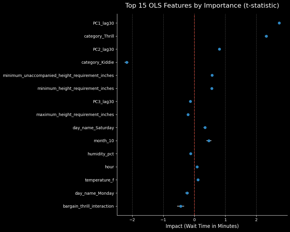
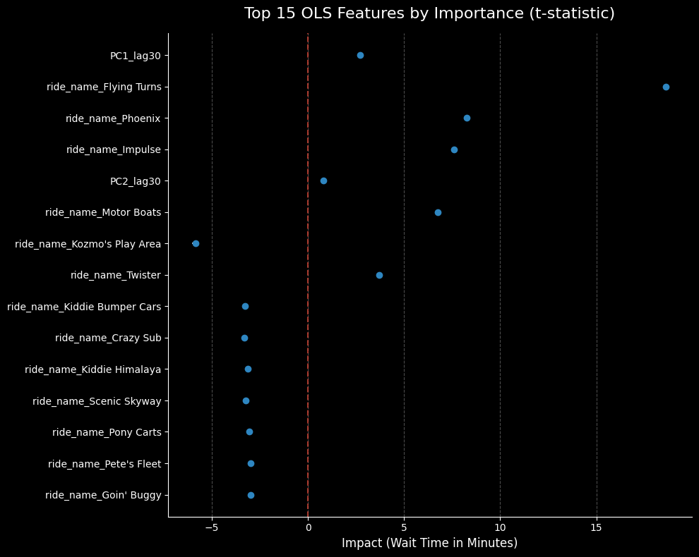
Because the continuous features — the lagged PCA components included — are z-scored, each coefficient reads in minutes per standard deviation. So the PC1_lag30 bar says: for every standard deviation of overall park busyness 30 minutes ago, the model adds ~2.7 minutes to its predicted wait for every ride at once. That uniform, parallel shift across the whole park is the same fingerprint that made PC1 "busyness" back in Part 1.Notice in the rides model on the right that Flying Turns is ranked second in importance, and the model just straight up adds 18 minutes to its estimated queue time. Period. Anyone who's waited in that line will corroborate it — and notice that's a flat add, applied no matter how dead the park is, which is the model's way of saying Flying Turns isn't slow because it's busy, it's slow because of how few it can load at a time.
Then trees: XGBoost, and why it isn't a forest
With a clean matrix and a readable OLS in hand, I moved to prediction proper — and to a completely different kind of model. This is also where the evaluation gets honest. OLS I fit on everything, because I'm using it to read its coefficients (inference). Every predictive model from here on uses a chronological 80/20 split — first 80% of time to train, last 20% to test. A random split would let the model train on the future and test on the past, which on time-series data is just leakage wearing a lab coat. (The random option lives in my code purely to demonstrate how flatteringly the metrics improve when I let it cheat.)
XGBoost is the opposite of OLS in almost every way. It never inverts a matrix; it makes logical if/then splits, so it shrugs off the dummy trap, collinearity, and NaNs entirely — it just ignores the redundant columns and splits on the rest. The thing I most wanted to understand was how it differs from a Random Forest, since both are "a bunch of trees." A Random Forest grows a crowd of deep, independent trees on bootstrapped samples and averages them — bagging, all at once, to cut variance. XGBoost grows its trees sequentially, each shallow tree fit to the errors the ensemble still has left over. And the "gradient" is literal: each new tree steps in the direction of the loss function's negative gradient, with learning_rate setting how big a step it's allowed to take down the mountain. It's gradient descent — partial derivatives and all — except the thing descending is the model itself.
Tuning those steps is where Bayesian optimization came in. Grid search is exhaustive and blind; Bayesian search builds a lightweight probability map of the error landscape (a Gaussian process) and balances exploration — testing blank regions — against exploitation — drilling into the known-good ones. It found strong hyperparameters in ~30 trials instead of 300, with Thomas Bayes and a little vector calculus on my side.
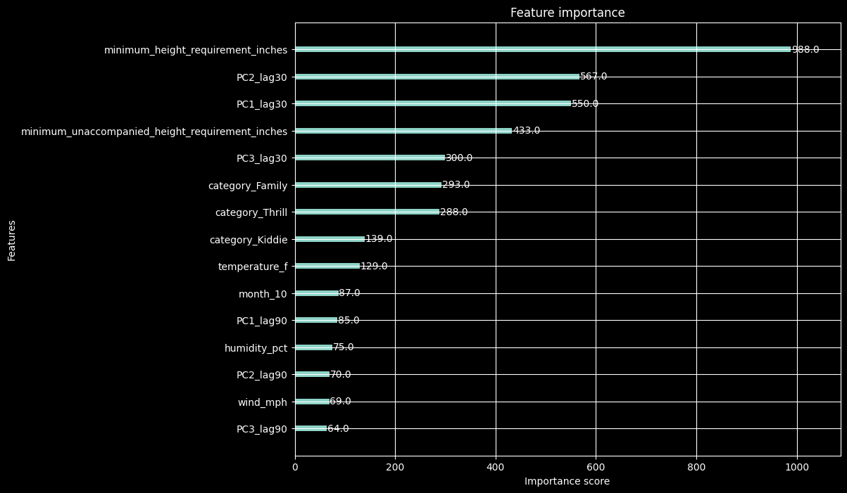
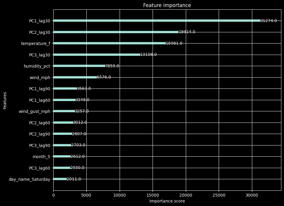
XGBoost feature importance, by split frequency — categories model (left) and rides model (right). Because trees ask yes/no questions instead of inverting a matrix, collinearity doesn't bite, so the 60- and 90-minute PC lags that wrecked the linear model get to stay — and the model uses them, reading the park's trajectory (filling up vs. emptying out) rather than a single 30-minute snapshot. The flavor flip is the interesting part: with each ride known by name (right), PC1_lag30 — overall busyness — is the single most-split feature; collapse identity down to Family/Thrill/Kiddie buckets (left) and minimum_height_requirement_inches jumps to #1, the model's best proxy for which ride is which once it can no longer name them. (Importance here is how often a feature is split on, which flatters many-valued continuous features over binary dummies — so weigh the continuous-vs-continuous bars as the fair ones.)
The idea that made a mess: lagging the PCA
By now XGBoost was giving genuinely good results, and I had a thought: I'd spent all of Part 1 distilling the park into three clean axes. Why not feed them back in as features?
The catch was immediate, and I caught it through the collinearity door before the leakage one. Each PC is a weighted blend of every ride's current wait — which means it's, almost by construction, highly correlated (if not flatly collinear) with the very matrix it was built from. Handing OLS a column that's a linear combination of columns it already has is the rank problem from the last section, in slow motion. The deeper reason is worse: that blend includes the wait for the exact ride I'm trying to predict, so the un-lagged PC doesn't merely correlate with the answer — it contains it. That's the leakage.
Lagging fixes both at once. "The state of the park thirty minutes ago" is something I actually know at predict time; it no longer contains the target row, and it's decorrelated enough from the present to stop poisoning the matrix. I lag at 30, 60, and 90 minutes so the model can read the trend — filling up versus emptying out — not just the level. How collinear are these things, really? Collinear enough that stacking the 60- and 90-minute lags on top of the 30 still blows up the OLS — so OLS and the net get only lag30, while XGBoost, which doesn't care, happily takes all three as a trend signal.
One bookkeeping point ate an afternoon. I align the lagged scores by timestamp — relabeling a score measured at $$S$$ as belonging to $$S + \text{lag}$$ — rather than by row offset, so the overnight close never bleeds yesterday's last reading into this morning's first row; a missing source bin just yields a NaN. (Opening-hour rows fill with 0, which isn't a fudge: PCA scores are mean-centered, so 0 literally means "average park state.")
First, textbook PCR replaces your predictors with components computed from those same predictors; here the components come from a different, wider matrix — the whole-park snapshot — and they're added on top of the real features, not swapped in for them.
Second, and this is the part that earns its keep: they're lagged. PCR has no concept of time. Lagging turns a contemporaneous summary of variance into a leading indicator — which is a forecasting move, not a dimension-reduction one. (And for two of the three models it isn't PCR by any definition, since trees and nets aren't linear regressions.)
There's even a flattering wrinkle. PCR's weak spot is that PCA is unsupervised — the highest-variance directions in your predictors aren't guaranteed to be the ones that predict the target. Here they are: the capstone shows PC1 (busyness) dominating every model. PCR hopes for exactly that alignment; I got to check it and watch it hold.
The clean experiment I haven't run yet is the genuine PCR setup: hand a model only the three lagged PCs and nothing else, and see how close it gets. The catch worth stating up front — with no ride identity, every ride looks identical at a given moment, so it can only predict park-level behavior. Which makes it a clean measurement of exactly one thing: how far "the whole park breathes together" gets you on its own. A good question for a Part 3.
And this is the point where the notebook became unmanageable. I was comparing rides-vs-categories and OLS-vs-XGBoost by commenting and uncommenting blocks of code — a thicket of dead branches whose state I kept having to hold in my head. So I stopped and built the actual pipeline: a chain of small pandas .pipe() steps that takes a flavor (rides or categories) and a type (ols, xgb, nn) and produces exactly the design matrix that combination needs.
df_model_ready = (df_raw
    .pipe(fill_height_nulls)
    .pipe(add_time_features)
    .pipe(add_lagged_pc_features, lagged_pcs, ...)
    .pipe(create_dummies, model_flavor=f)
    .pipe(encode_weather, model_type=t)
    .pipe(add_promo_features, model_flavor=f)
    .pipe(standardize_numerics, model_type=t)
    .pipe(finalize_df, model_flavor=f, model_type=t)
)
XGBoost comes out with raw dummies and its NaNs intact; OLS and the net come out standardized, single-lagged, with reference baselines dropped. The pipeline wasn't foresight — it was me cleaning up a mess I'd already made.
An idle curiosity: the neural net
The neural network started as a what-if, and then I decided that if I was going to include it I'd tune it properly — every choice measured, not vibed, all on the same chronological split and averaged over several seeds. (Seeds matter: there's ~0.1 min of run-to-run jitter even at a fixed seed, so single-run comparisons lie.)
Two transforms do almost all the work:
| input X | target y | mean MAE |
|---|---|---|
| raw | raw | 3.04 |
| standardized | raw | 2.54 |
| raw | log1p | 2.42 |
| standardized | log1p | 2.17 |
The log1p on the target is the big lever. Wait times are heavily right-skewed (skew ≈ 3.4), which wrecks the MSE landscape; the log cuts MAE ~28% and converges ~10× faster, and expm1 inverts it so predictions come back in honest minutes.
Then the genuinely counterintuitive result — smaller networks won:
| architecture | params | mean MAE |
|---|---|---|
| (128, 64) | 19,841 | 2.40 |
| (64, 32) ← my first guess | 7,873 | 2.12 |
| (32, 16) | 3,425 | 2.00 |
| (16, 8) | 1,585 | 1.96 |
| (8, 4) | 761 | 1.98 |
MAE falls as the net shrinks, bottoming out at a tiny (16, 8). Capacity was never the constraint: even the largest net I tried, ~20k parameters against ~600k training rows, sees about 30 rows per parameter — far too little room to overfit. The extra neurons just give Adam more ways to wander into a worse minimum. The final net is ~7% more accurate than my first guess with five times fewer parameters — and the smallness pays off later, because a 16-neuron hidden layer is something you can actually read.
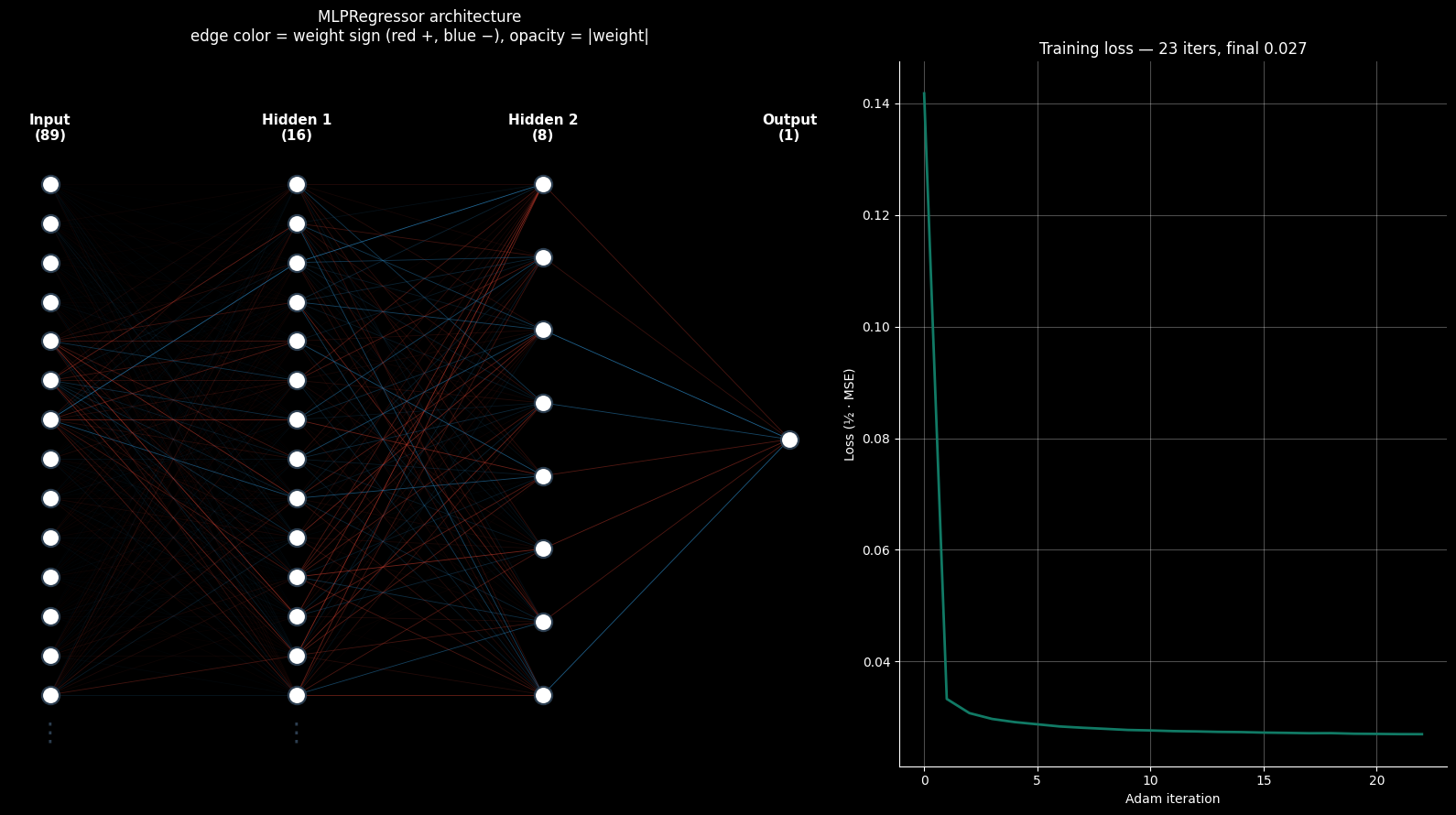
log1p target — the internal objective, not minutes). That steep-then-flat shape is the dividend of standardizing the inputs and logging the target: a clean loss landscape Adam can fall straight down.The bake-off
Here's the part that surprised me. After tuning, all three model families land within a rounding error of each other — XGBoost and the net effectively tie at around 1.97 MAE, under two minutes of average error on a quantity that's only ever posted in five-minute increments, and the linear model isn't far behind. Three completely different machines, roughly the same wall.
Once they tie on accuracy, accuracy stops being the interesting axis — interpretability takes over. OLS hands you its coefficients but can only add. XGBoost is robust to everything but speaks in thousands of opaque splits. The net bends to anything but buries its reasoning in a tangle of weights. So the rest of this post is less "which model wins" and more "which model will tell me what it learned — and did any of them learn what I learned in Part 1?"
One honest negative result
Before the good part, one dead end I want to mention. I tried using a neural net not as the predictor but as an unsupervised feature compressor — a deep tanh autoencoder squeezing all ~89 features through a narrow bottleneck ("PCA, but it can bend"), then handing only the latent codes to XGBoost. The bet was that nonlinear codes might surface an interaction the trees couldn't already find.
They didn't. XGBoost with the autoencoder codes (2.03) was no better than XGBoost on the raw matrix (2.01). The learned codes added nothing, so the autoencoder is retired. I mention it because a portfolio that only shows what worked is a portfolio lying by omission.
Capstone: putting my Part 1 interpretations on trial
This is the part I'm most pleased with, because it applies Part 1's own method — form a reading, then try to falsify it against something the model never saw — one level up. The three lagged park-state PCs visibly dominated every model once I added them. So I ran a mediation A/B: fit the rides OLS without the lagged PCs, then with them — same rows, same other features — and watched what moved. If my Part 1 stories about PC1/PC2/PC3 were right, the displacement should follow a predictable pattern.
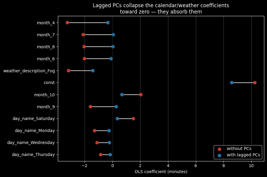
The logic: the PCs are lagged park state, sitting causally downstream of the calendar and the weather. It's the Saturday and the pleasant October afternoon that cause the crowd thirty minutes later. So if a PC is a good summary of "how busy is it," adding it should absorb the coefficients of whatever was merely proxying for crowd state — day of week, month, weather — while leaving the ride-identity coefficients alone, since each PC is one number per snapshot, identical for every ride in a bin.
That's exactly what happened for PC1. Three columns alone produce a real jump in R^2, and the displacement is clean: ride-identity coefficients barely move, while the calendar and weather coefficients collapse toward zero — roughly 13× more drift. The PCs soaked up the proxies for crowd state and left the ride signal untouched. PC1 lands as the dominant term in the after-model with an enormous t-statistic, and the direction of its correlations holds the Part 1 reading up: busiest on Saturdays, busiest in October, busiest when it's cooler — fall weekends, not the dead heat of August. Busyness, confirmed and strengthened. PC2 behaves as expected too: it barely engages here, because its meaning lives in ride-space, not in the calendar — consistent with the spatial reading.
What the PCs absorbed
| without_PCs | with_PCs | |
|---|---|---|
| month_4 | -3.253 | -0.345 |
| month_7 | -2.091 | 0.048 |
| month_8 | -2.048 | 0.029 |
| month_6 | -2.017 | -0.114 |
| weather_description_Fog | -3.204 | -1.428 |
| const | 10.271 | 8.599 |
| month_10 | 2.005 | 0.665 |
| month_9 | -1.597 | 0.269 |
| day_name_Saturday | 1.484 | 0.356 |
| day_name_Monday | -1.291 | -0.255 |
| day_name_Wednesday | -1.241 | -0.284 |
| day_name_Thursday | -0.864 | -0.16 |
What each PC proxies
Correlations of each lagged PC with the interpretable features (read the rankings, not magnitudes — a binary dummy can't correlate hard with a continuous axis). PC1 = busyness holds up (Saturdays, October; busiest when cooler → fall weekends, not hot summer). PC2 is weak here because it's a spatial contrast living in ride-space. PC3 tracks weather more than hour — see the ride-description deep-dive below for its real meaning.
| PC1_lag30 | PC2_lag30 | PC3_lag30 | |
|---|---|---|---|
| temperature_f | -0.304 | 0.135 | -0.282 |
| day_name_Saturday | 0.297 | 0.053 | 0.008 |
| month_10 | 0.255 | 0.104 | -0.042 |
| month_6 | -0.188 | 0.112 | -0.042 |
| month_7 | -0.179 | 0.032 | -0.169 |
| day_name_Monday | -0.17 | 0.01 | -0.035 |
| day_name_Wednesday | -0.157 | -0.008 | -0.028 |
| month_8 | -0.146 | 0.03 | -0.087 |
| day_name_Thursday | -0.133 | -0.013 | -0.057 |
| day_name_Friday | 0.102 | -0.197 | 0.165 |
| humidity_pct | -0.085 | -0.037 | 0.079 |
| day_name_Tuesday | -0.075 | 0.092 | -0.045 |
| wind_mph | 0.064 | -0.034 | 0.2 |
| precipitation_in | -0.056 | -0.008 | -0.008 |
| weather_description_Thunderstorm | -0.054 | 0.001 | 0.017 |
| wind_gust_mph | 0.052 | -0.093 | 0.156 |
| sundown_special | -0.052 | -0.062 | -0.003 |
| weather_description_Overcast | 0.051 | -0.14 | 0.069 |
| weather_description_Partly cloudy | -0.046 | -0.031 | -0.019 |
| hour | 0.038 | 0.151 | -0.137 |
| cloud_cover_pct | -0.037 | -0.142 | 0.045 |
| weather_description_Mainly clear | -0.03 | 0.053 | -0.039 |
| month_4 | -0.028 | 0.015 | 0.023 |
| month_9 | -0.021 | 0.111 | -0.096 |
| weather_description_Fog | -0.012 | -0.002 | 0.004 |
| bargain_night | 0.004 | -0.042 | -0.012 |
| bargain_thrill_interaction | 0.002 | -0.014 | -0.002 |
PC3: killing another of my own pretty hypotheses
Part 1 ended with a lesson I was rather smug about: be willing to throw out an attractive hypothesis. I'd earned it by junking my first PC3 story (ride throughput) in favor of a clean time-of-day reading. Part 2 made me eat it, because the daypart story was the next attractive hypothesis — and it doesn't hold up either.
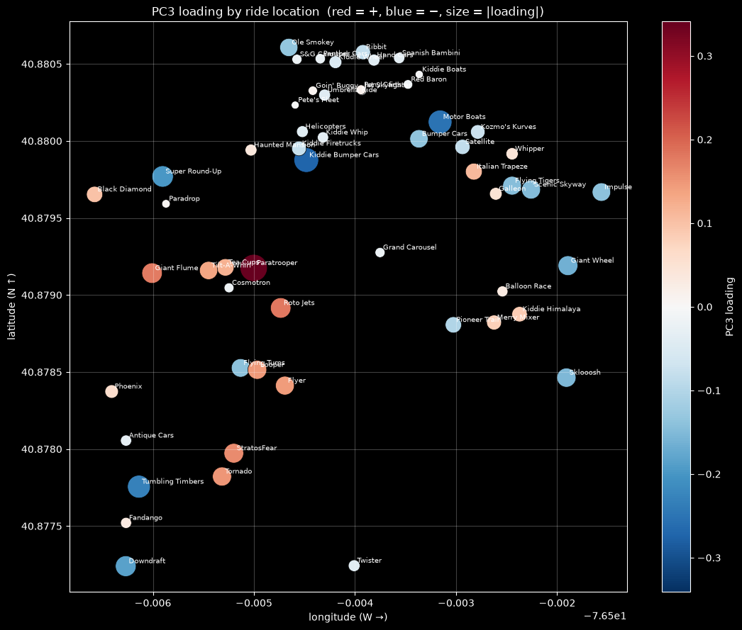
With 60 rides and a pile of ride-attribute data I scraped from Knoebels' own WordPress REST API — descriptions, GPS, water-vs-dry, height, install year, duration, intensity, speed — I went back at PC3 properly. It correlates more with ride intensity (r ≈ 0.35) and with weather than it does with hour. When the capstone fed it the daypart hypothesis to absorb, it shrugged. So I'm explicitly ruling out daypart — along with ride age, water, and pure geography. The cleanest read I can offer now is fast spinning, whirling flats ↔ slow transport and water rides, but at 7% of the variance it's a weak, only-loosely-interpretable axis. I had it cleaner in Part 1; I had it cleaner and wrong.
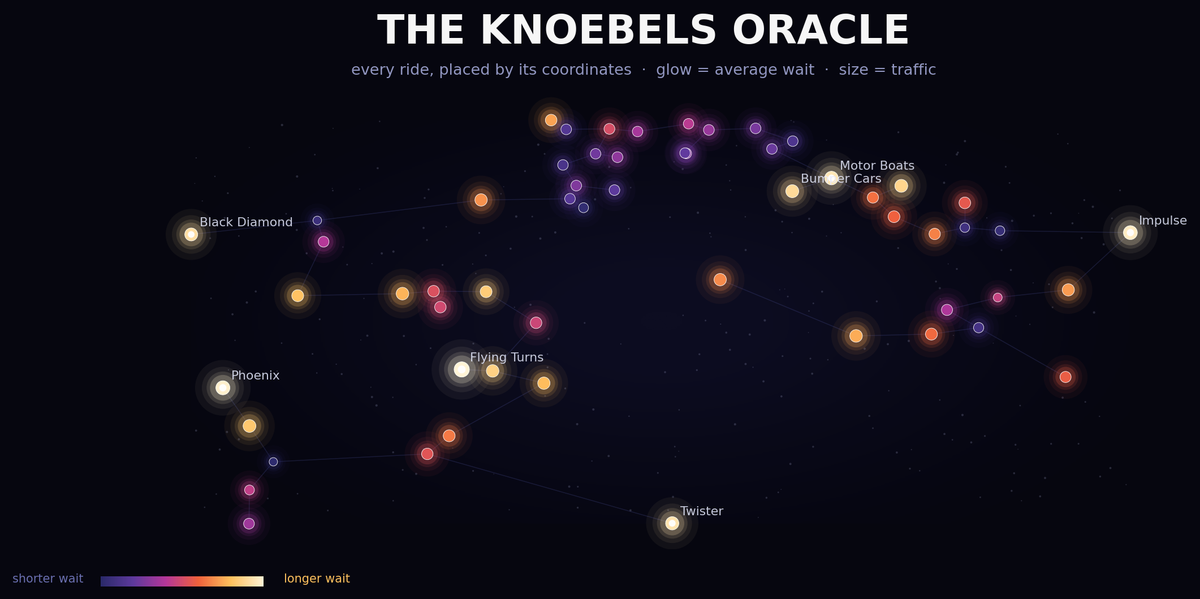
So, an open invitation. Below is a map: every ride at its real latitude and longitude, colored by its PC3 loading. The spinning flats cluster loosely in the central midway and the blues ring the periphery, but there's no crisp rule. If you know Knoebels and you see the pattern I missed, I'd genuinely love to hear it.
Scrying the neural net
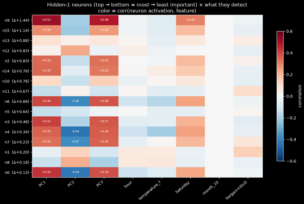
This is where the Oracle nickname earns its keep. The tuned XGBoost and the net tie on accuracy — but only one of them lets me pry it open. Each of the net's 16 first-layer neurons is a learned weighted blend of the 89 inputs: a loading vector, exactly like a PCA component. So I can read them the way I read PC1/PC2/PC3 — inspect the weights, correlate each neuron's activations with interpretable features, and ablate each one (switch it off, measure the damage) to find which ones actually carry the prediction.
The punchline: the network independently elevated "how busy was the park 30 minutes ago" to a top internal feature. One neuron tracks PC1 strongly, and ablation ranks it among the most important of the sixteen. With no knowledge of my PCA, gradient descent reached for the same signal the linear model leaned on hardest. Two completely different model families, one discovery — the same busyness axis I'd extracted by hand a season earlier.
There's even a visible division of labor in the layer: one neuron turns out to be a ride-memorizer — the bulk of its weight sits on specific ride dummies, and it ignores park-state entirely — while others specialize in the global crowd signal. The net quietly split its sixteen neurons between "which ride is this" and "how busy is the park," which is roughly how I'd have drawn the problem on a napkin.
The honest caveat, since this whole post runs on them: because PC1's lag is itself an input, a neuron leaning on it isn't a from-scratch rediscovery. The non-trivial result is that ablation puts those park-state neurons at the top — and, unlike PCA's clean orthogonal axes, the net smears busyness across several neurons instead of isolating one. Fuzzier than PCA, but unmistakably the same concept.
What I took away
- The hard part of a forecaster is proving you're not cheating. The PCA features were dangerous twice over — collinear because they're derived from the matrix, and leaky because they contain the target — and lagging defused both.
- Starting with statsmodels OLS was the best pedagogical decision in the project. It forced me to stare at condition numbers and VIFs and actually understand the matrix, where scikit-learn would have silently run anything.
- Accuracy converged; interpretability didn't. Three model families landed within a rounding error (~1.97 MAE), which turned the interesting question from which is best into which will explain itself.
In Part 1 I read the park's mind. In Part 2 I tried to build a copy of it — and the strange, satisfying part is that the copy, assembled by gradient descent with no idea what a roller coaster is, kept reaching for the same first thought I did: how busy is it right now?