How does semantic search actually work anyway?

First let me hedge a little bit: there are many and much better resources for learning about this topic. Three Blue One Brown will rotate your brain in nicer ways. Anything by Jay Alammar is a clearer picture than I'm about to draw. But explaining something is the best way to review and cement your own knowledge, so here goes.

I've written a few posts now about the Obsidian-RAG-pipeline (clunky moniker such that it is) — what it does, what it unlocks, how it's implemented. But I've sort of been waving my hands at the bottom layer. How does the search part actually work?

Turns out the answer is: a tiny bit of linear algebra (the best algebra), and one matrix multiplication.

A vector is just a list of numbers

Take v = (3, 4) and w = (4, 3). In 2D these are arrows from the origin out to those coordinates. Two arrows that obviously aren't pointing in exactly the same direction, but are leaning in roughly the same general direction.

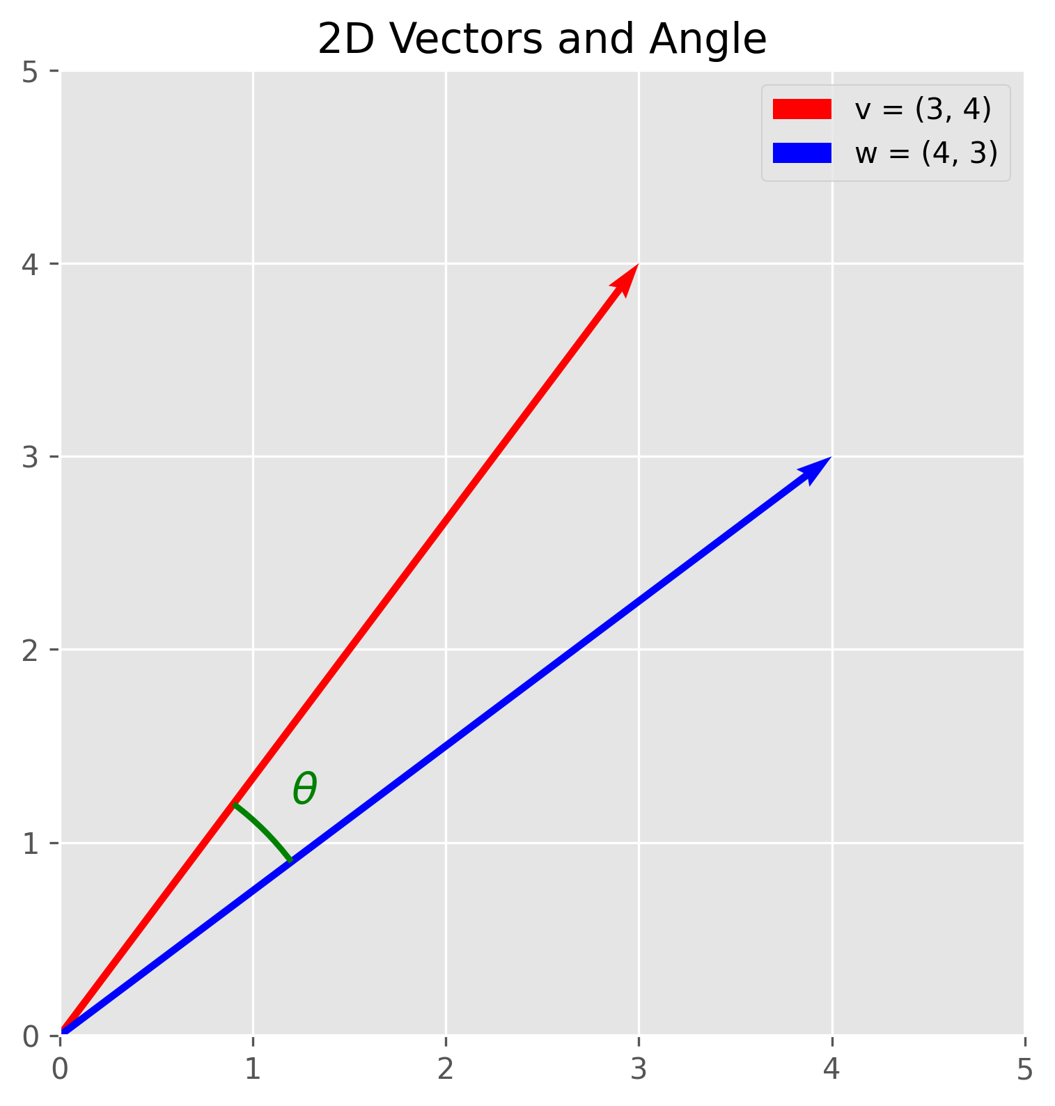
We want a way to put a number on "how similar are the directions these two arrows are pointing?" The tool for this is the dot product, which has two equivalent definitions:

• The component formula: v · w = v₁w₁ + v₂w₂ + ...
• The geometric formula: v · w = |v| · |w| · cos θ, where |v| means "the length of v"

The fact that those two formulas describe the same thing is genuinely cool and worth a moment. The components-and-multiply version is mechanical; the geometric version says it's secretly about the angle. They're the same.

Combining them gives us cosine similarity:

cos θ = (v · w) / (|v| · |w|)

Working it out for our example:

v · w = (3)(4) + (4)(3) = 12 + 12 = 24

|v| = √(3² + 4²) = √(9 + 16) = √25 = 5
|w| = √(4² + 3²) = √25 = 5

cos θ = 24 / (5 · 5) = 24/25 = 0.96

θ = arccos(0.96) ≈ 16.26°

If √(3² + 4²) = 5 rings a bell, that's because the 3-4-5 right triangle is the same one stamped into every carpenter's speed square. Length of a vector is just Pythagoras with delusions of grandeur.

So v and w are about 16 degrees apart, and the cosine of that angle is 0.96 — close to 1, which is what we'd get if they were perfectly parallel. Cosine similarity ranges from 1 (parallel — same direction, maximally similar) through 0 (perpendicular, also called orthogonal — no relationship) to -1 (anti-parallel — pointing opposite directions). Hold onto that orthogonality case; it's going to come back hard when we get to 768 dimensions.

Dot product vs. cosine similarity

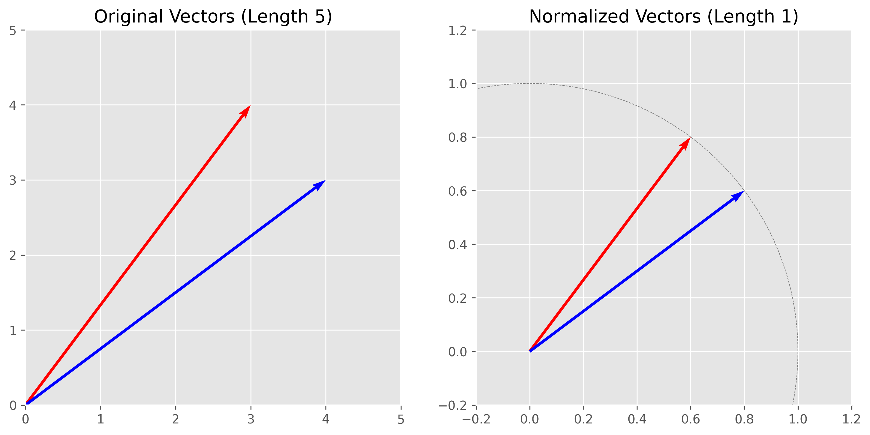
These often get talked about as if they're rival concepts, but they're really not. Cosine similarity is just the dot product divided by the magnitudes. If you do some upfront work and normalize your vectors to unit length first — divide each by its own magnitude — then the magnitudes are both 1 and the dot product is the cosine similarity. No division step at query time.

Normalizing our example: v becomes (0.6, 0.8), w becomes (0.8, 0.6), and (0.6)(0.8) + (0.8)(0.6) = 0.96. Same answer, but now obtainable in a single dot product. This is what every embedding model and vector database does under the hood: store unit vectors so that similarity search collapses to one multiply-and-add per pair.

That's the linear algebra you need. Two arrows, an angle between them, a single number that quantifies how parallel they are.

What's an embedding?

Spoiler: an embedding is a vector.

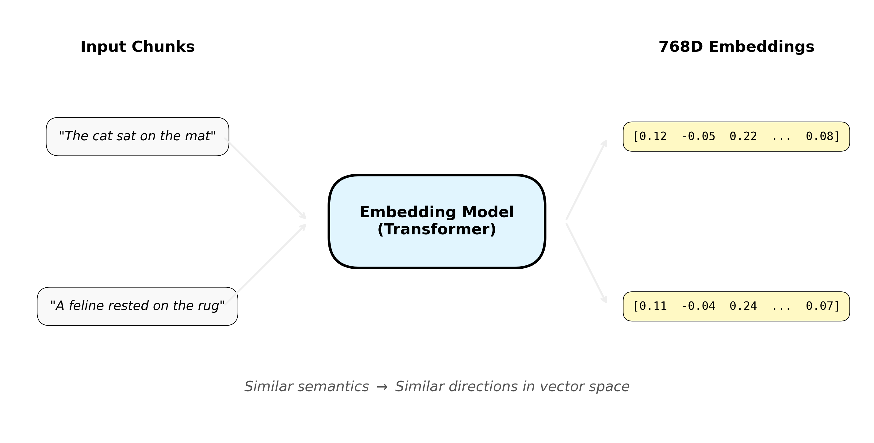
The whole job of an embedding model is to take some piece of input — a chunk of text, an image, an audio clip — and produce a fixed-length vector such that semantically similar inputs come out pointing in similar directions. That's it. That's the whole trick. The cleverness is in the training; the output is just numbers.

Most text embedding models I've used (bge, nomic-embed-text, e5) produce 768-dimensional vectors. So the sentence "the cat sat on the mat" goes in, and 768 numbers come out. Those 768 numbers, taken together, point somewhere in 768-dimensional space — or, as I prefer to call it, 768-dimensional Lovecraftian hellspace, because high-dimensional geometry is genuinely alien in ways your 3D-trained intuition will get wrong. No single dimension is meaningful on its own — you can't ask "what does dimension 47 mean?" and get a clean answer. But the direction of the whole vector encodes meaning. Sentences about cats sitting on things will end up pointing roughly the same way. Sentences about Roman history will point a totally different way.

Here's where that orthogonality case from earlier comes back to do real work. In 768-dimensional space, two random unit vectors are almost certainly nearly perpendicular to each other. The math of high-D space pushes everything toward orthogonality by default — there's just so much room for vectors to be unrelated to each other that "unrelated" is the overwhelmingly likely outcome when you pick at random. So when two embeddings do come back with a high cosine similarity, that's not a coincidence and it's not noise. The model has done real work to place those two pieces of text near each other against the statistical pressure for everything to be orthogonal to everything else. Similarity in high dimensions is earned. That's the property that makes semantic search work at all: when your query vector ends up pointing the same way as some chunk vector in this hellspace, that alignment is meaningful, because random alignment essentially never happens.

The contrast with what's happening inside an LLM

Worth pausing on this because it explains why semantic search is cheap and LLM inference is not.

When a frontier LLM reads your prompt, every token gets its own vector — and tokens are often sub-word pieces. The word "embedding" might be split by byte-pair encoding (BPE) into "em" and "bedding," each of which is its own token, each of which gets its own vector. Sentence-embedding models tokenize the same way under the hood — usually with WordPiece or BPE — but their vocabularies tend to be smaller than frontier LLMs', not larger. BERT-derived models like bge use a ~30k-token WordPiece vocab; Llama 3 uses 128k BPE; the bigger frontier vocabs are an investment LLM teams have made specifically to keep sequence lengths down on long prompts.

The more interesting difference isn't the tokenizer, it's what the model has learned the tokens to mean — and how much it gets to figure that out in context. A frontier LLM resolves "MI" on the fly through attention: its many layers consult the surrounding tokens ("patient", "presented with", "cardiac") and pull the meaning of that token toward myocardial infarction; in a different prompt full of state names and highway exits, the same model pulls it toward Michigan instead. Contextual disambiguation is one of the main jobs attention does, and frontier LLMs have an enormous amount of attention to throw at it.

Embedding models have attention layers too — modern ones are transformer-based — but the output of that whole stack gets pooled into one 768D vector per chunk and frozen. Whatever disambiguation happened during that single forward pass is baked into the vector; there's no second-chance contextual resolution at query time. A general-purpose embedding model with weak medical priors might handle "the patient presented acutely with MI" okay because the chunk has enough surrounding context for its attention to lean on, but a one-word chunk of just "MI" will land squarely in Michigan-land. A clinical-domain embedding model has seen "MI" enough in patient-care contexts that its attention has learned to default toward the medical meaning, and the frozen vectors land closer to the right neighborhood even when context is sparse. This is why picking a domain-appropriate embedding model matters when your corpus is specialized — the tokenizer rarely fails you, but the learned semantics will if the model wasn't trained on data that looks like yours.

Anyway: those token vectors then flow through dozens of attention and feed-forward layers, each one rewriting the vectors based on context, before the final layer projects the result back into vocabulary space to pick the next token. Hidden dimension in something like Llama 3.1 405B is around 16,384, and the model has hundreds of billions of parameters spread across all those layers. Per-token compute is enormous. This is why frontier inference wants H100s and embedding models will happily run on your laptop.

A sentence-embedding model pays its (much smaller) cost exactly once per chunk, stores the resulting vector, and reuses it forever. That's most of why semantic search is cheap at runtime: the expensive part already happened and got cached as 768 floats.

From a chunk to an index

In practice you don't embed whole documents. You chunk them. A chunk is some unit of text — a paragraph, a section heading and its body, a fixed token-count window — small enough to be coherent, large enough to be meaningful. Chunking strategy is its own deep rabbit hole (semantic chunking, recursive character splitting, sentence-window, parent-document retrieval) and gets its own post one of these days. For now, just know that you decide on some splitting scheme and end up with N chunks.

Each chunk gets embedded. Now you have N pairs of (chunk_text, 768-dim vector). You need to store them somewhere that supports fast nearest-neighbor lookup. Two options I've used:

FAISS — Facebook's library. In-memory, blazing fast, supports HNSW/IVF for sub-linear search at large N. Great if your data fits in RAM and you're okay with the operational overhead of "I now have a binary index file to manage alongside whatever stores the actual text."

pgvector — Postgres extension that adds a vector column type, similarity operators (<=> for cosine distance), and ANN indexes via HNSW or IVFFlat. SQL all the way, plays nice with all your other relational data, scales fine for any corpus a personal project is going to hit. This is what powers the Obsidian-RAG-pipeline.

Either way, the data structure underneath is conceptually the same: a big matrix where each row is one chunk's embedding.

The actual search is one matrix multiplication

This is the part I think is underrated by most "intro to embeddings" content.

Setup: your index is a matrix A with shape (N, 768) — N chunks, each a 768-dimensional row. Your query, after running through the same embedding model, is a vector q with shape (768,). Both have been unit-normalized.

The search is:

similarities = A @ q

The result is a vector of shape (N,). Each entry is the cosine similarity between the query and one chunk. Take the top-k entries — those are your search results. The ones with cosine closest to 1 are the chunks pointing most similarly to the query.

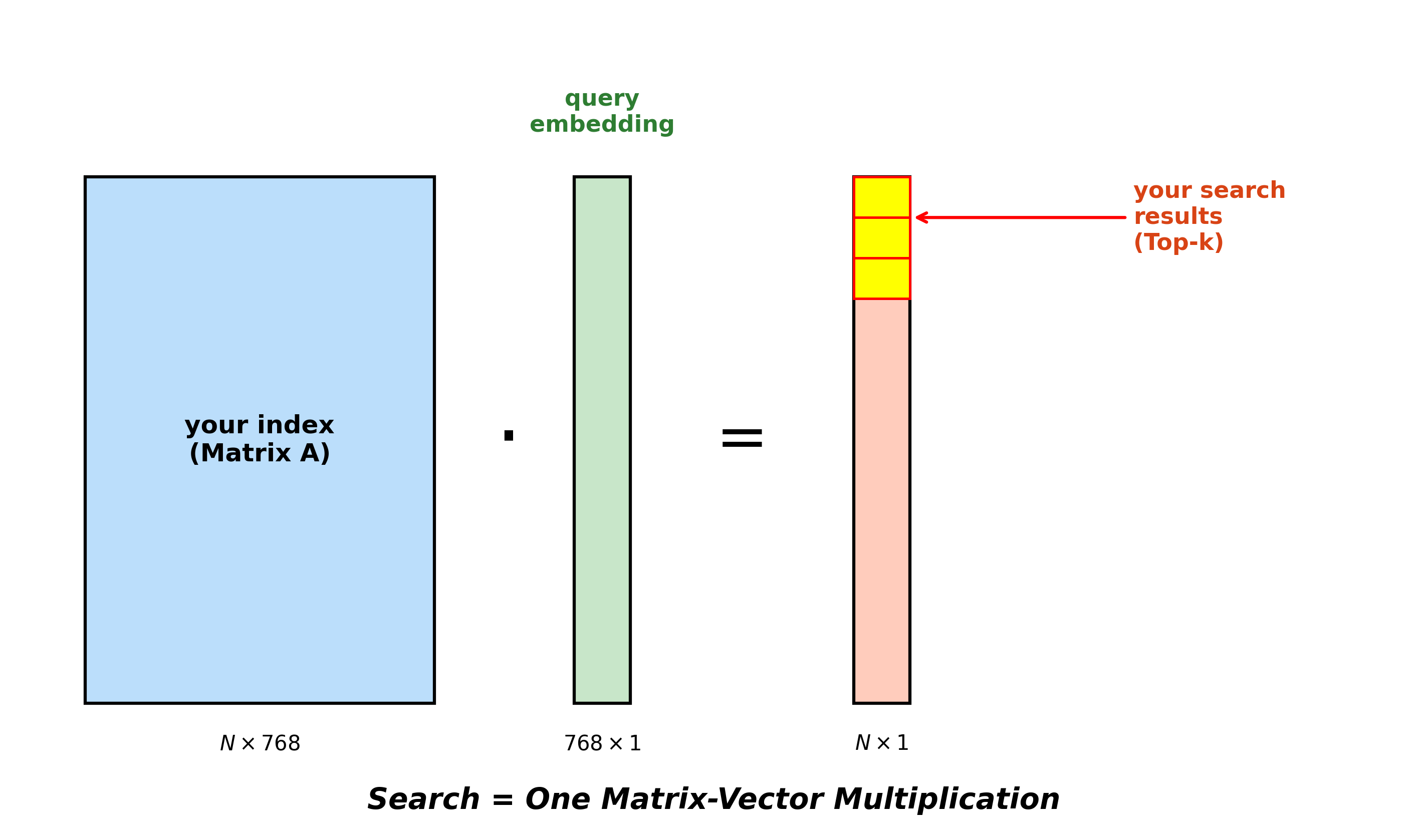
That's it. That is the entire algorithm.

There is depth in any direction you want to look — approximate nearest neighbor algorithms (HNSW, IVF, product quantization) for when N is in the millions and you can't afford the full matmul per query; hybrid retrieval that combines this with BM25; rerankers that take the top-50 results and re-score them with a smarter (slower) model — but the core operation is one matrix-vector product.

There's also a reason this scales beautifully. GPUs are matrix multiplication accelerators. Whether your index has ten thousand vectors or a hundred million, the shape of the work is the same; you just hand a bigger matrix to the same hardware. The whole modern vector-search infrastructure is built on top of "the thing GPUs are best at, we already need to do."

What this looks like

Words only get you so far. Linear algebra wants to be drawn.

Below is a 3D projection of every chunk currently in my Obsidian-RAG pgvector index. Each dot is one chunk; hover for the text. I've also pre-embedded a handful of example queries you can click through — each one shows up as a red point with lines drawn to its top-5 nearest chunks by cosine similarity (computed in the original 768D space, not the cartoon 3D version you're looking at). You can toggle the projection between PCA and UMAP, and the difference between the two is itself part of the lesson — more on that in a second.

(I went with pre-embedded queries because exposing my self-hosted embedding endpoint to the public internet gave me agita. The pedagogical payoff is the same either way — you can see what "top-k by cosine similarity" actually looks like when the query and the index live in the same vector space.)

A couple of caveats this thing is hiding from you:

Remember the bit earlier where I said no single dimension of the embedding is meaningful on its own — that "dimension 47" isn't a thing you can name? PCA is what you get when you take that observation seriously. The principal components aren't any of the original 768 axes; they're new directions through the 768D space, each one a weighted combination of all 768 original dimensions, chosen so that the first one captures the most variation in your data, the second captures the most of what's left, and so on. Meaning lives in directions through the space, not along whichever axes the model happened to write its output to. PCA's entire job is to find those directions and rank them. The PCA view in the viz above is what you get when you keep the top three.

The toggle gives you two very different pictures of the same data. PCA is linear and deterministic: it finds the directions of greatest variance in the embedding space and projects onto the top three. Same vectors in, same picture out, every time. It preserves global shape — what's far from what — but clusters can look smushed together because PCA isn't trying to separate them, just to spread the data out along the axes of widest variation. UMAP is nonlinear and stochastic: rather than chasing variance, it tries to preserve local neighborhood relationships using a graph-based approach, and tends to give you visibly tighter, more separated clusters. The catch is that re-running UMAP with a different random seed gives you a different layout — the clusters that emerge are real, but their absolute positions in 3D space aren't meaningful the way PCA's are. Toggle between them in the viz and you'll see this firsthand: a chunk that's at one position under PCA can be in a completely different spot under UMAP, but its neighbors will be largely the same.

Neither one is "right." They're answering different questions. PCA answers "what are the major axes of variation in this data?" UMAP answers "what's near what?" Both are fair questions to ask of your embedding space.

Also: yes, projecting from 768 dimensions down to 3 sounds insanely lossy, and at first blush the math agrees — keeping the top 3 of 768 PCA components feels like throwing away over 99% of your information. But there's a saving grace baked into how embedding models actually distribute meaning. The 768 dimensions are not all equally loaded. Most of the meaningful variation in your corpus lives on a much-lower-dimensional manifold inside the ambient 768D space — the model isn't using all 768 axes uniformly to encode the differences between your chunks. Since the principal components are sorted by how much variation each one captures, keeping the top 3 captures more than the naive "0.4% of dimensions" math suggests, because the lower-ranked dimensions weren't doing much work to begin with. (UMAP gets at the same underlying structure from a totally different angle, which is why both projections, despite looking different, will agree about which chunks are near which.)

So yes, the projection is heavy. But it's not random destruction. We three-dimensional beings get a fair-enough peek at the high-dimensional structure, as long as we remember the picture is a shadow of the thing, not the thing itself.

This is also a nice place to mention that the linear-algebra-as-pictures muscle I built up doing a pygame cube rotation exercise earlier this year is exactly what made this viz feel approachable. Both exercises are the same thing — apply a matrix to a bunch of vectors, render the result, learn to see the operation. The cube was 8 vertices in 3D rotated by a 3×3 matrix. This is N chunks in 768D projected by a 768×3 matrix. Same picture, different scale.

Wrapping up

The whole story:

• Vectors and dot products give us a way to ask "how parallel?" in any number of dimensions.
• Embedding models give us vectors whose directions encode meaning.
• Storing a corpus of those vectors gives us a big matrix.
• Searching is one matrix-vector multiply, plus a top-k.

There's depth in every direction — the training of the embedding models themselves, hybrid search that combines dense vectors with BM25, ANN indexing for huge corpora, rerankers, chunking strategies, the question of why high-dimensional space is genuinely weird in ways that matter for all of this. Posts for another time.

If you want to go deeper on the linear algebra, the obvious move is Gilbert Strang's MIT 18.06 — the lecture videos are free on YouTube and the textbook is the textbook. 3Blue1Brown's Essence of Linear Algebra series is the visual companion. Between them, every "huh, why does that work" question has an answer waiting for you.