Everyday I'm shufflin, part 1: Where did all of the indexes go?
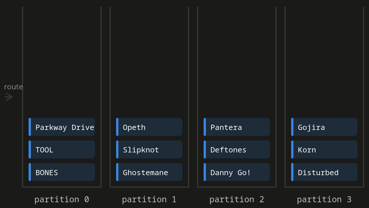
There's one line of pseudocode that made distributed joins click for me and it's embarrassingly simple:
partition_number = floorMod(hash(join_key), N)That's the shuffle. Every machine runs that same function over every row it's holding, and every row with the same join key ends up on the same machine no matter where it started. Once that's true each machine can join its own slice without knowing anything about anybody else's data, and you just concatenate the results.
The line is old. Dean and Ghemawat wrote it into the MapReduce paper in 2004, basically verbatim:
Reduce invocations are distributed by partitioning the intermediate key space into R pieces using a partitioning function (e.g., hash(key) mod R).
— MapReduce: Simplified Data Processing on Large Clusters, §3.1
A few paragraphs later, in §4.1, they note that the default hash partitioner "tends to result in fairly well-balanced partitions," which is funny because most of this post is about breaking that.
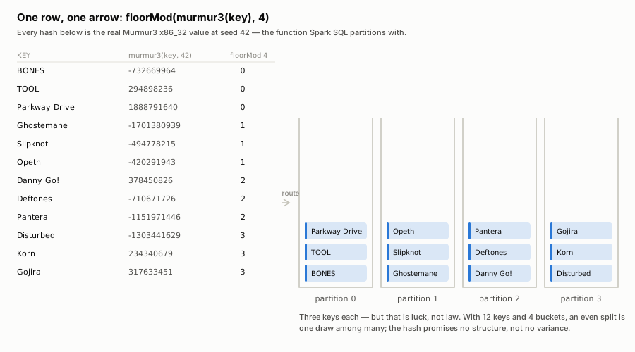
I ended up writing (an analogue of) the whole thing in Java to convince myself I understood it. Partitioner, executor threads, barrier, sort, merge, roughly four hundred lines. The data is my own Spotify listening history, about 71,000 plays sitting in Postgres, which turned out to be a much more interesting choice than I expected and not for the reason I picked it.
Why not just use an index?
If you write SQL for a living the shuffle looks like a step backwards. You already know how to make a join fast: index one side, let the optimizer do a nested loop. For each of N outer rows, seek into a B-tree of M inner rows. O(N log M), and the inner table never gets scanned or sorted or materialized.
That's a great plan and it's great because every one of those seeks is cheap. A B-tree seek is a few pointer chases through pages that are probably already in the buffer pool.
Now put the inner table on forty machines. The naive translation is "for each outer row, ask the cluster where the matching row lives, and go get it." But look at what that's actually asking. Which machine has this key? A B-tree can't answer that. A B-tree tells you where a row sits in a file on the machine you're already standing on. It has nothing to say about which machine you should have asked in the first place.
So you need a second index, over machines, keyed by the join key. And that index is a hash function. Which means it isn't really a second index at all. In a shared-nothing cluster the index and the data placement are the same decision.
The RDD paper states this, in the middle of a taxonomy of dependencies:
map leads to a narrow dependency, while join leads to wide dependencies (unless the parents are hash-partitioned).
— Resilient Distributed Datasets, NSDI 2012, §4
That parenthetical is the whole shebang. A join is expensive unless the data was already partitioned by the join key, in which case it's free. Spark ships this as a feature: bucketed tables and Storage Partition Join exist to skip the shuffle entirely, and when SPJ fires "the query plan will not contain Exchange nodes prior to the join."
Which gives you this framing which really made it crystal clear for me:
A shuffle is the index, built at query time, because nobody built it at write time.
Bucketing is the distributed version of a clustered index. Shuffling is what happens when there isn't one. And Spark is explicit that these are the same mechanism, in the comment above the hash expression that drives both:
/**
 * A MurMur3 Hash expression.
 *
 * We should use this hash function for both shuffle and bucket, so that we can
 * guarantee shuffle and bucketing have same data distribution.
 */
case class Murmur3Hash(children: Seq[Expression], seed: Int) extends HashExpression[Int] {
  def this(arguments: Seq[Expression]) = this(arguments, 42)
Same function, same seed, whether the partitioning happens now or happened last Tuesday when somebody wrote the table.
Then it sorts, usually. But why?
The obvious answer is "so it can do the merge join," and for Spark's sort-merge join that's correct. I want to poke at it anyway because the interesting question is why Spark reaches for a sort-based join at all when it has a hash-based one sitting right there.
It does. ShuffledHashJoinExec takes the same shuffle, builds a hash table from the smaller partition, probes it. No sort anywhere. If sorting weren't for the merge, Spark would just use that and skip an O(n log n) step on every partition.
So why is sorting the default? Spark says so itself, in the config that decides:
prefer sort merge join over shuffled hash join. Sort merge join consumes less memory than shuffled hash join and it works efficiently when both join tables are large.
—spark.sql.join.preferSortMergeJoininSQLConf.scala, defaulttrue
Memory. A hash join has to hold one side's whole partition resident. A sort-merge join streams both sides and spills when it has to, so its memory is bounded no matter how big that partition turns out to be.
So, lets restate that: The planner picks a strategy before the shuffle runs, from estimates. If one partition turns out to hold 3.4 million rows when the average holds 125,000 (in part two, one does) a hash join on that partition runs out of memory. A sort-merge join just gets slower.
The sort is insurance against skew. You pay O(n log n) on every partition to survive the one partition you couldn't predict.
You can watch Spark drop the insurance once it doesn't need it anymore. maxShuffledHashJoinLocalMapThreshold lets the planner switch to a hash join when AQE's runtime stats prove every partition is small, which is knowledge it didn't have when it first planned the query.
Two places where the sort genuinely isn't about joining, and they matter in part two: a GROUP BY has to bring a key's rows together before it can reduce them, and a window function's ORDER BY is so obvious it almost doesn't bear mentioning. There's no hash-based alternative that produces row numbers.
The crack in "fairly well-balanced"
Hashing balances keys. It says nothing about rows. And rows per key, in every real dataset I've ever worked with, is a power law.
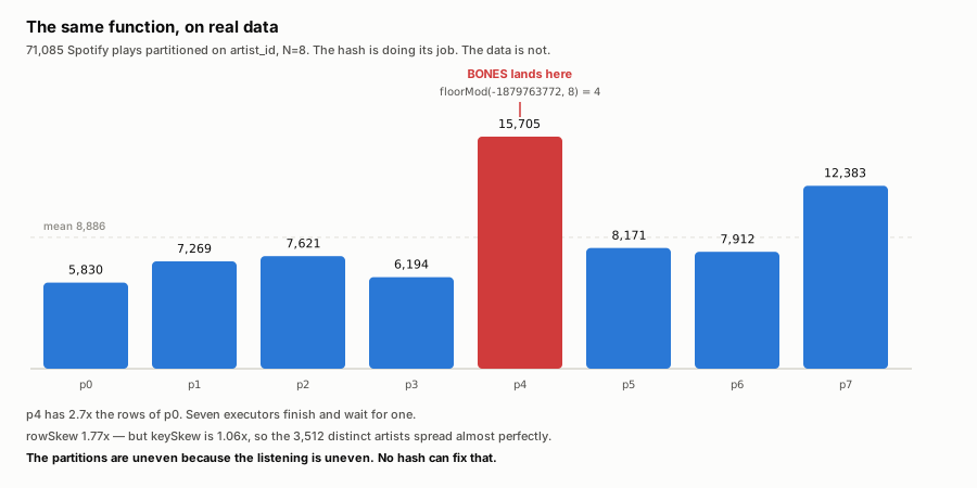
That's 71,085 real plays across eight partitions, hashed with Spark's own function. Partition 4 holds 15,705 rows, partition 0 holds 5,830. Seven executors finish and wait for one.
The hash isn't at fault and I can show it. Measured over distinct keys instead of rows, the worst partition is 1.06× the mean. The 3,512 artists spread almost perfectly. It's the plays that are lumpy. One artist, BONES, is 12.9% of everything I've ever listened to, and those rows can't be split across two machines because they all have to meet the same artist row.
Which is a straggler, in the sense the MapReduce authors defined twenty-two years ago:
One of the common causes that lengthens the total time taken for a MapReduce operation is a "straggler": a machine that takes an unusually long time to complete one of the last few map or reduce tasks.
— §3.6
And they'd already named the distribution, buried in the section motivating combiners:
Since word frequencies tend to follow a Zipf distribution, each map task will produce hundreds or thousands of records of the form<the, 1>. All of these counts will be sent over the network to a single reduce task…
— §4.3
A Zipf distribution producing a hot key that swamps one reducer. When I fitted my own artist play counts the exponent came out at α = 0.85 with R² = 0.968.
So the hot key problem isn't a bug and it isn't new. It's the documented cost of the design.
Four keys, four different ways to break
| Key | Distinct | Top share | What breaks |
|---|---|---|---|
track_id |
12,258 | 0.54% | nothing, this is the control |
primary_artist_id |
3,512 | 12.9% | one hot key, one straggler |
owner_id |
2 | 73.3% | 6 of 8 partitions get zero rows |
is_rap (derived) |
3 | 52.0% | parallelism capped at 3 |
is_rap is mine, I designed it intentionally to cause skew issues for this exercise. There's no such column in the mart. I derived it by regex over each artist's genre list (rap|hip hop|trap|phonk|drill) with a third value for the 11.9% of plays whose artist has no genres at all. The genre data underneath is real, the column is a construction.
I kept it because the failure it produces is one I'd never properly thought about, and because a derived low-cardinality flag isn't exotic. It's a status column, a country code, a tier, an is_active. People group on these constantly.
And it breaks differently from a hot key. is_rap is nearly balanced, 52/36/12, no dominant value at all. But with three distinct values and eight partitions, five executors get nothing, and adding cores can't help. No hash spreads three values across eight buckets, and raising the partition count makes it worse: now you have 197 empty partitions instead of 5.
Rows are the wrong unit
So I, like most of us I imagine, tend to think of the data in terms of rows. I'd been reporting skew as a row ratio. Partition 4 has 15,705 rows against a mean of 8,886, so 1.77×. Clean number, easy to reason about, and not what Spark looks at.
Every threshold that governs this is denominated in bytes:
| Setting | Default | What it decides |
|---|---|---|
autoBroadcastJoinThreshold |
10 MB | broadcast the small side instead of shuffling |
coalescePartitions.minPartitionSize |
1 MB | floor on a coalesced partition |
advisoryPartitionSizeInBytes |
64 MB | target when splitting a skewed partition |
skewJoin.skewedPartitionThresholdInBytes |
256 MB | below this, a partition is never "skewed" |
None of them count rows, for good reason. Rows aren't a fixed size. Ten million integers and ten million JSON blobs are the same row count and four orders of magnitude apart in just about every other way.
So I added bytes to the stage report. It computes the serialized size arithmetically rather than actually serializing, which is fast but only useful if it's right, so there's a test that serializes twenty thousand rows for real and asserts the arithmetic matches to the byte:
private static long serializedSize(Play play) {
    return utf(play.playId())
            + 8                       // playedAt, epoch millis
            + utf(play.ownerId())
            + utf(play.trackId())
            + utf(play.albumId())
            + utf(play.artistId())
            + 4                       // durationMs
            + 1;                      // rapClass ordinal
}
Two caveats about what that number isn't: Spark compares against shuffle block sizes from MapStatus, which are bytes on disk after compression, and which are stored log-quantized: compressSize rounds each block up to the next power of 1.1, so the sizes AQE reasons about are good to about 10% and biased high. My numbers are an uncompressed upper bound on a quantity that's itself fuzzy. Treat every crossover below as an order of magnitude, not a decimal.
What my data actually weighs
key=ARTIST  partitioner=spark-murmur3  N=200
total=71,085  min=19  mean=355  max=9,958
rowSkew=28.02x (max/mean)   vsMedian=53.83x (AQE's test)   keySkew=1.77x
shuffleWrite=9.3 MB  biggestPartition=1.3 MB
9.3 MB. That's the whole fact table. Every song I have ever streamed, serialized, is smaller than a photo off my phone. And the biggest partition, the one holding BONES, the straggler this entire project is about, is 1.3 MB.
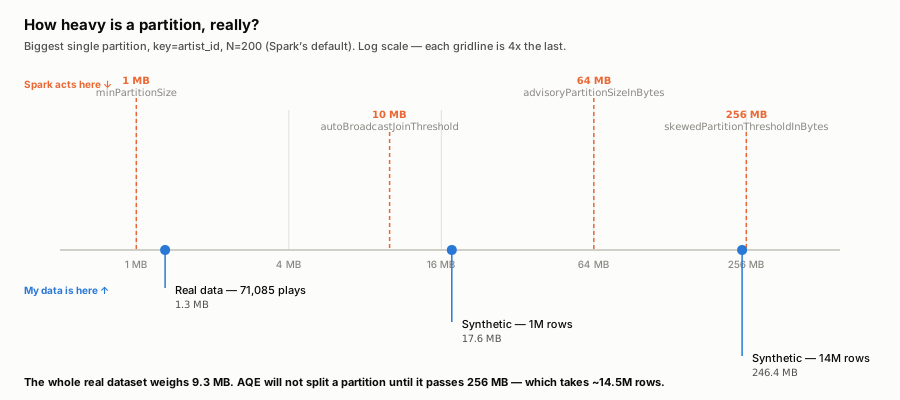
For scale, that 9.3 MB total is the same order as the 10 MB default for broadcasting a dimension. The thing I've been calling the big side of the join is about the size of the small side Spark would decide not to shuffle at all.
AQE needs two conditions and skew is the easy one
Spark's adaptive skew handling has been on by default since 3.2.0 and the docs describe it in a sentence:
Spark dynamically handles skew in sort-merge join by splitting (and replicating if needed) skewed partitions.
The definition of "skewed" is where it gets interesting:
A partition is considered as skewed if its size is larger than this factor multiplying the median partition size and also larger thanskewedPartitionThresholdInBytes.
— factor default 5.0, threshold default 256 MB
Both, not either. So run my data past it:
| Condition | Gate | My data | |
|---|---|---|---|
| skew factor | > 5.0× median | 53.83× | passes, 10.8× over |
| partition size | > 256 MB | 1.3 MB | fails, 197× under |
The most skewed dataset I own clears Spark's factor ten times over and is 197 times too small for Spark to look at it. The hot key is real, the straggler is real, and AQE sits there with its hands in its pockets. Correctly, too. Splitting a 1.3 MB partition costs more in scheduling than it could possibly save.
That's not a flaw in the threshold, that's the threshold working. Skew only costs you when the skewed thing is big.
Where it actually starts to matter
The skew is a property of the distribution, not the row count, so I can hold the shape fixed and turn up the volume. N=200 throughout, which is Spark's default.
| Rows | Shuffle write | Biggest partition | vs median | Passes 256 MB? |
|---|---|---|---|---|
| 71,085 (real) | 9.3 MB | 1.3 MB | 53.8× | no |
| 1,000,000 | 130.7 MB | 17.6 MB | 39.9× | no |
| 10,000,000 | 1.28 GB | 176.0 MB | 40.2× | no |
| 14,000,000 | 1.79 GB | 246.4 MB | 40.3× | no, by 9.6 MB |
| 25,000,000 | 3.19 GB | 440.2 MB | 40.2× | yes |
| 50,000,000 | 6.38 GB | 880.7 MB | 40.3× | yes |
Look at the skew column. It doesn't move. ~40× at a million rows, ~40× at fifty million. Of course it doesn't, the distribution is the same and a ratio doesn't care about scale.
Everything else moves, and the byte column is what decides Spark's behavior. Somewhere around 14.5 million rows the same workload that Spark ignored becomes a workload Spark actively rewrites. That's a discontinuity at a point that has nothing to do with your data.
Which means "is my job skewed?" and "will Spark do anything about it?" are different questions.
But I'm one guy
The obvious objection to all of this is that 71,000 plays is a toy. Fair. Except the missing dimension isn't time, it's users. I'm one listener. The table already has two.
| Users like me | Plays | Shuffle write | Hot partition |
|---|---|---|---|
| 1 | 71 K | 9.3 MB | 1.3 MB |
| 200 | 14.0 M | 1.79 GB | 256 MB, the gate |
| 1,000 | 71 M | 9.1 GB | 1.3 GB |
| 10,000 | 711 M | 90.8 GB | 13 GB |
200 users. Not a hundred thousand, not a million. About the headcount of a mid-sized company, and Spark starts rewriting your query plan. Ten thousand users, which is a rounding error against Spotify's actual user base, puts the hot partition at 13 GB.
So "my data is 200× too small" doesn't mean this scenario is exotic. It means a single-tenant slice of a normal multi-tenant fact table sits just under the threshold.
(One caveat I'll mark as reasoning rather than measurement: the byte volume scales linearly with users and that part's certain. Whether the hot key stays at 12.9% depends on how correlated people's taste is, and my BONES is not everyone's. But global music consumption is itself a power law, so if anything the skew sharpens with scale.)
So is my job skewed?
For my data, yes. One artist is 12.9% of the plays, the biggest partition is 53.8× the median, and at eight partitions seven executors finish and wait for the eighth. That's skew by any definition I'd put my name to.
Will Spark do anything about it? No, and it's right not to. The whole fact table is 9.3 MB and the hot partition is 1.3 MB, against a gate of 256 MB. The skew ratio barely moves as the data grows, the bytes do, and only the bytes get Spark's attention.
So they really are different questions, and at my scale they get opposite answers. Part two is about what the straggler actually costs once it's big enough to matter, and the skew AQE never looks at because it isn't in a join.
Appendix: the hash, and seed 42
A quick aside on the hash, because I lost a few hours to it. Spark SQL uses Murmur3 x86_32 at seed 42, thenPmod(a positive modulo) against the partition count. I went to grab an implementation off the shelf, and you shouldn't. Murmur3 eats its input in 4-byte blocks, and when the length isn't a multiple of four Spark handles the leftover bytes differently than everyone else does. It runs each trailing byte through the full block step where standard Murmur3 folds them in once. Spotify IDs are 22 characters. 22 % 4 = 2. So every single key in my dataset hashes differently under Spark than under Commons Codec or Guava. BONES' artist ID comes out-1879763772under Spark and-1619811190under standard Murmur3.
This got filed as a bug (SPARK-23381) and the resolution is the interesting part: they added a compatible variant alongside and left the original alone, with a comment saying to keep it "for backward compatibility for the components existing before 2.3." Of course they did. Go back and read that Murmur3Hash comment again. Every bucketed table on disk was written with the old behavior. Fixing the hash would silently stop those tables matching the shuffle that reads them.
Seed 42, by the way, has been there since the expression was born (SPARK-12480, Wenchen Fan, January 2016). The doc comment carefully explains what the seed is for and says nothing about its value. Thirty-six comments on that PR, not one of them asks. Guava, which Spark's implementation is based on, seeds with 0. So long, and thanks for all the fish.
Sources
- Dean & Ghemawat, MapReduce, OSDI 2004 — §3.1 partitioning and sort, §3.6 stragglers, §4.1 partitioning function, §4.3 the combiner and Zipf
- Zaharia et al., Resilient Distributed Datasets, NSDI 2012 — §4 narrow vs wide dependencies
- Spark source:
Murmur3_x86_32.java,hash.scala,SQLConf.scala - SPARK-23381 (Murmur3 tail divergence), SPARK-12480 (seed 42)
- Spark SQL Performance Tuning docs for every threshold default quoted above